my blog

I’m a big fan of the CamScanner app and have been using this program on my phone ever since a friend introduced it to me many years ago. You take a snapshot of a piece of paper and CamScanner will produce a pdf with crisp, very readable, text and the background removed. I wanted to add this functionality to my cam_board script (the name is homage to CamScanner) and after a lot of experimentation I believe I finally have a simple solution. Below is a description of the resulting procedure. It is an abridged version of the algorithm inside cam_board. The line numbers correspond to the denoise.py file available here.

import argparse
import cv2
import numpy

The argparse library will be used to parse the command line arguments. This might be overkill since there will be only one argument - the name of the image (without the extension) that will undergo the denoising procedure. The cv2 library in conjunction with the numpy library will be used to perform image manipulations.

Next the single command line argument is parsed and it will be available in args.input [denoise.py line: 42]

parser = argparse.ArgumentParser(description = "Denoise image.")
parser.add_argument("input" , help = "Input image name (without extension)")
args = parser.parse_args()

Note that the image name is expected not to contain the extension, e.g.instead of warped1.png the command line expects warped1.

warped = cv2.imread(args.input + ".png")

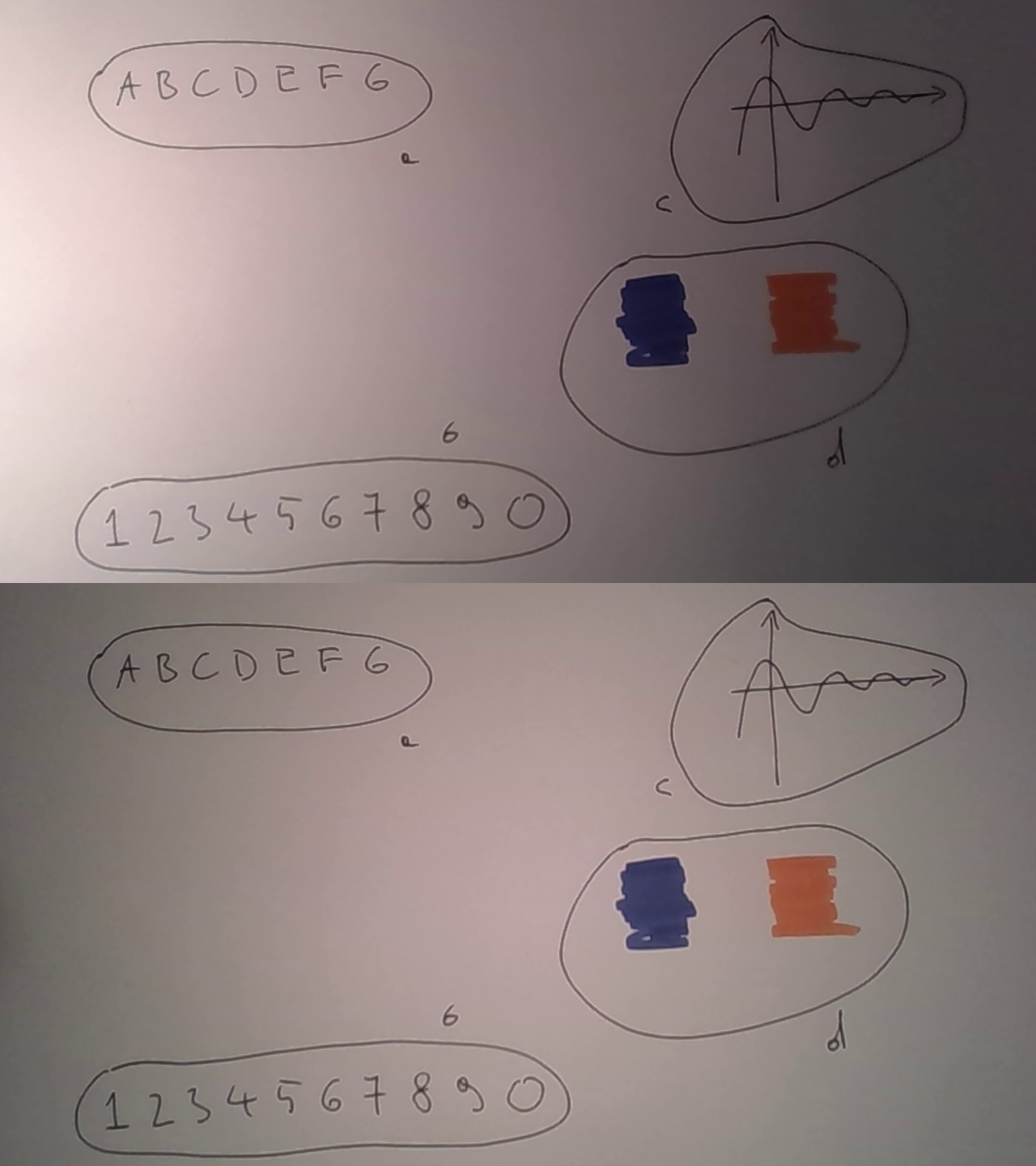
The denoise repository contains four sample images: warped1...4.png that were “warped” inside cam_board (web cam frames are morphed so that four special markers showing up on a printout are stretched to the four corners of the image). Here we will use warped1.png and warped4.png. Each image contains some text (a), some numbers (b), a simple graph (c) and two patches of color (d).

Notice that the the image on the top has the light shining on it differently then the image on the bottom.

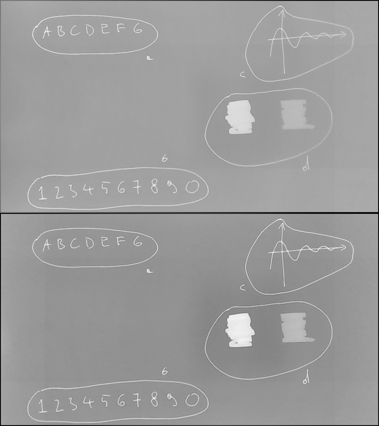
In the next step the image is turned into grayscale (cv2.COLOR_BGR2GRAY) [denoise.py line: 88]

gray = cv2.cvtColor(warped , cv2.COLOR_BGR2GRAY)

Dark areas of the image will be treated as the “signal” and pixels in these areas should have hight color values. This is achieved through color inversion [denoise.py line: 91]

gray = 255 - gray

cv2.imwrite(args.input + "_gray.png" , gray)

Now it is time to take care of the background. But first, the gray image will be turned into a floating point array [denoise.py line: 124]

gray = gray.astype("float32")

This is usefull since we are about to apply many floating operations to this array of pixels.

blur_kernel = numpy.ones((300 , 300) , dtype = numpy.float32) 
blur_kernel = blur_kernel / numpy.sum(blur_kernel.flatten())

Notice that in the second line it is divided by the number of elements (albeit not in the most efficient way :-), I’ll have to fix this in cam_board) and applied to the gray image [denoise.py line: 133]

blured_gray = cv2.filter2D(gray , -1 , blur_kernel)

At this point blur_kernel contains a moving average. The value of each pixel in this array is an average of \(300 \times 300\) surrounding pixels. This intermediate result is written to a file [denoise.py line: 137]

cv2.imwrite(args.input + "_blured_1.png" , blured_gray)

My experimets show that it is beneficial to erase a three pixel wide boarder around the image [denoise.py line: 153]

gray[0:3 , :] = 0.0
gray[gray.shape[0] - 3 : gray.shape[0] , :] = 0.0
gray[: , 0:3] = 0.0
gray[: , gray.shape[1] - 3 : gray.shape[1]] = 0.0

blured_gray = cv2.filter2D(gray , -1 , blur_kernel)

cv2.imwrite(args.input + "_blured_2.png" , blured_gray)

This helps get rid of any artifacts that might be on the edges of the image but has a sideffect in the form of ghosting on the border of the blured images:

Next, the gray image is shifted relative to the estimated background blured_gray. This helps with evening out the different lighting conditions in different parsts of the image [denoise.py line: 180]

gray_2 = (gray - blured_gray)
gray_2 = 255.0 * (gray_2 - numpy.amin(gray_2)) / (numpy.amax(gray_2) - numpy.amin(gray_2))
cv2.imwrite(args.input + "_gray_2.png" , gray_2)

Additionally, the standard deviation of gray-blured_gray image is calculated: [denoise.py line: 186]

stdv = numpy.sqrt(numpy.mean(((gray - blured_gray) * (gray - blured_gray)).flatten()))

and this value will be used as a metric to classify an image pixel as the “signal” or as the “noise”.

Pixels that are classified as “signal” will retain their shade of color but will have modified brightness depending on the “signal” strength. There is an infinite number of ways to do this but my experiments convinced me that it is best to first transform the image to the HLS color space [denoise.py line: 201]

hls = cv2.cvtColor(warped , cv2.COLOR_BGR2HLS)

Next in order to adjust brightness and leave the original shade of color only the L channel is changed [denoise.py line: 205]

h_res = hls[: , : , 0]
l_res = numpy.full(gray.shape , 255.0 , dtype = numpy.float32)
l_res = numpy.where((gray - blured_gray) > stdv , hls[: , : , 1] , l_res)
s_res = hls[: , : , 2]

Finally, the resulting image is reconstructed (cv2.merge) and converted to blue-green-red (cv2.COLOR_HLS2BGR) colorspace [denoise.py line: 226]

warped = cv2.cvtColor(cv2.merge((h_res.astype("uint8") , l_res.astype("uint8") , s_res.astype("uint8"))) , cv2.COLOR_HLS2BGR)

cv2.imwrite(args.input + "_warped.png" , warped)

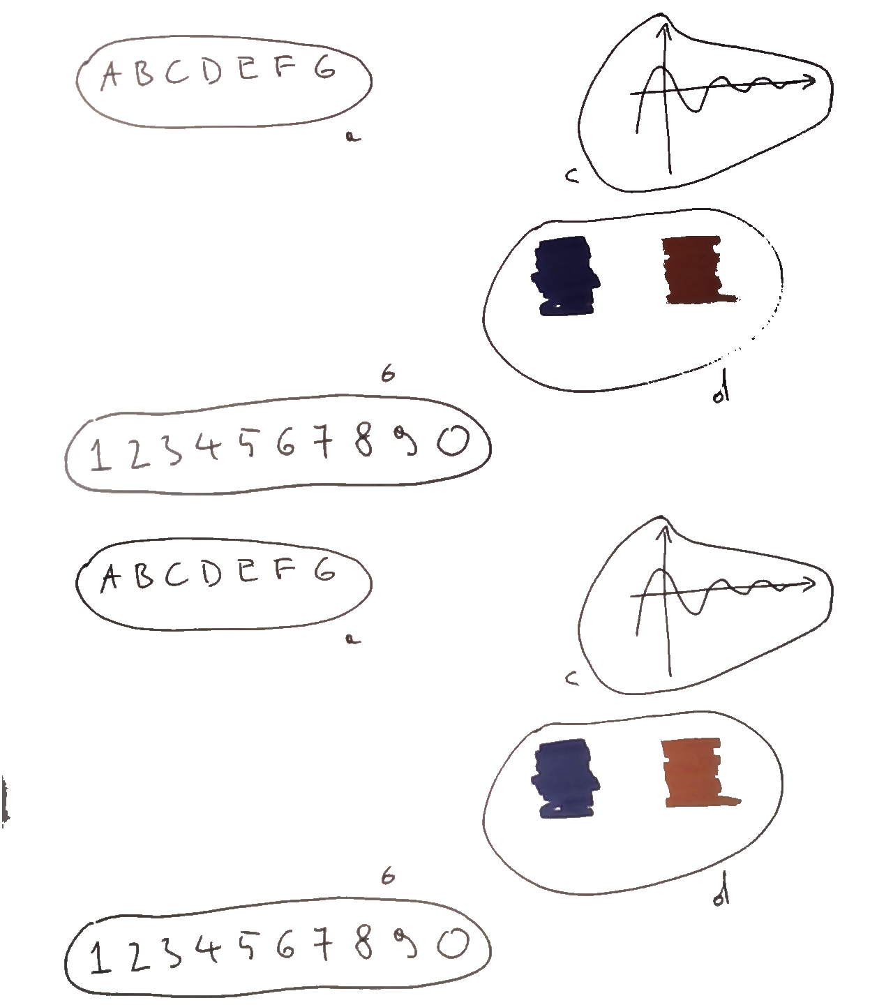
Personally, I think this looks alright. The letters (a), numbers (b), graph (c) are crisp and sharp. The color patches (d) on the look more vibrant then the ones on the top, probably due to better lighting conditions. There are some problems with this approach however. If the bluring kernel size (currently set to 300 by 300) is smaller then larger color patches will appear vibrant on the edges and faded in the middle.

image denoising with python